Firstly, let’s generate a dataset with continous data.

set.seed(1)

(rand_data<-round(c(rnorm(5,10,2),rnorm(5,80,4)),0))

##  [1]  9 10  8 13 11 77 82 83 82 79

JMP

We can use JMP to fit the smooth curve model in JMP which has another name Kernel Density Estimation. Then we can use this model to calculate the quantile.

R

Of course, you have another choice to finish this work with R. there’re sereval ways to do this.

Details refer to Wikipedia

Option 1

You can use density function in stat package to fit estimate the model and used as a parameter in function quantile.density in spatstat package to calculate the quantile.

library(spatstat)

## Loading required package: spatstat.data

## Loading required package: nlme

## Loading required package: rpart

## 
## spatstat 1.59-0       (nickname: 'J'ai omis les oeufs de caille') 
## For an introduction to spatstat, type 'beginner'

## 
## Note: R version 3.5.1 (2018-07-02) is more than 9 months old; we strongly recommend upgrading to the latest version

quantile.density(density(rand_data),c(0.00135,0.5,0.99865))

##    0.135%       50%   99.865% 
## -46.63139  45.30272 137.63139

Option 2

You canalso use density function in stat package to fit estimate the model and use uniroot function to calculate the root result which. sometimes, the result is the same with JMP, if it is not consist with the result in JMP, it may be caused by the bw value, and you can specify the bw value to get the same value. Of course, the result in JMP is not the “correct result”, you can calculate the quantile with appropriate method.

quantile_kde<-function(z,p=.95,bw=density(z)$bw){
  g <- function(x, z, bw, p) sum(pnorm(x-z, sd=bw))/length(z) - p
  uniroot(g,range(density(z)$x)+c(-1,1),z=z,bw=bw,p=p)$root
}

for(i in c(0.00135,0.5,0.99865)){
  cat(sprintf("The %f quantile is %f\n",i,quantile_kde(rand_data,i)))
}

## The 0.001350 quantile is -48.703622
## The 0.500000 quantile is 45.357844
## The 0.998650 quantile is 139.628200

Option 3

There’s a function to calculate the kde funciton

set.seed(1)
data = c(rnorm(100,-10,1),rnorm(100,10,1))
 
phi = function(x) exp(-.5*x^2)/sqrt(2*pi)
 
tpdf = function(x) phi(x+10)/2+phi(x-10)/2
 
h = sd(data)*(4/3/length(data))^(1/5)
 
Kernel2 = function(x) mean(phi((x-data)/h)/h)
 
kpdf = function(x) sapply(x,Kernel2)
 
x=seq(-25,25,length=1000)
 
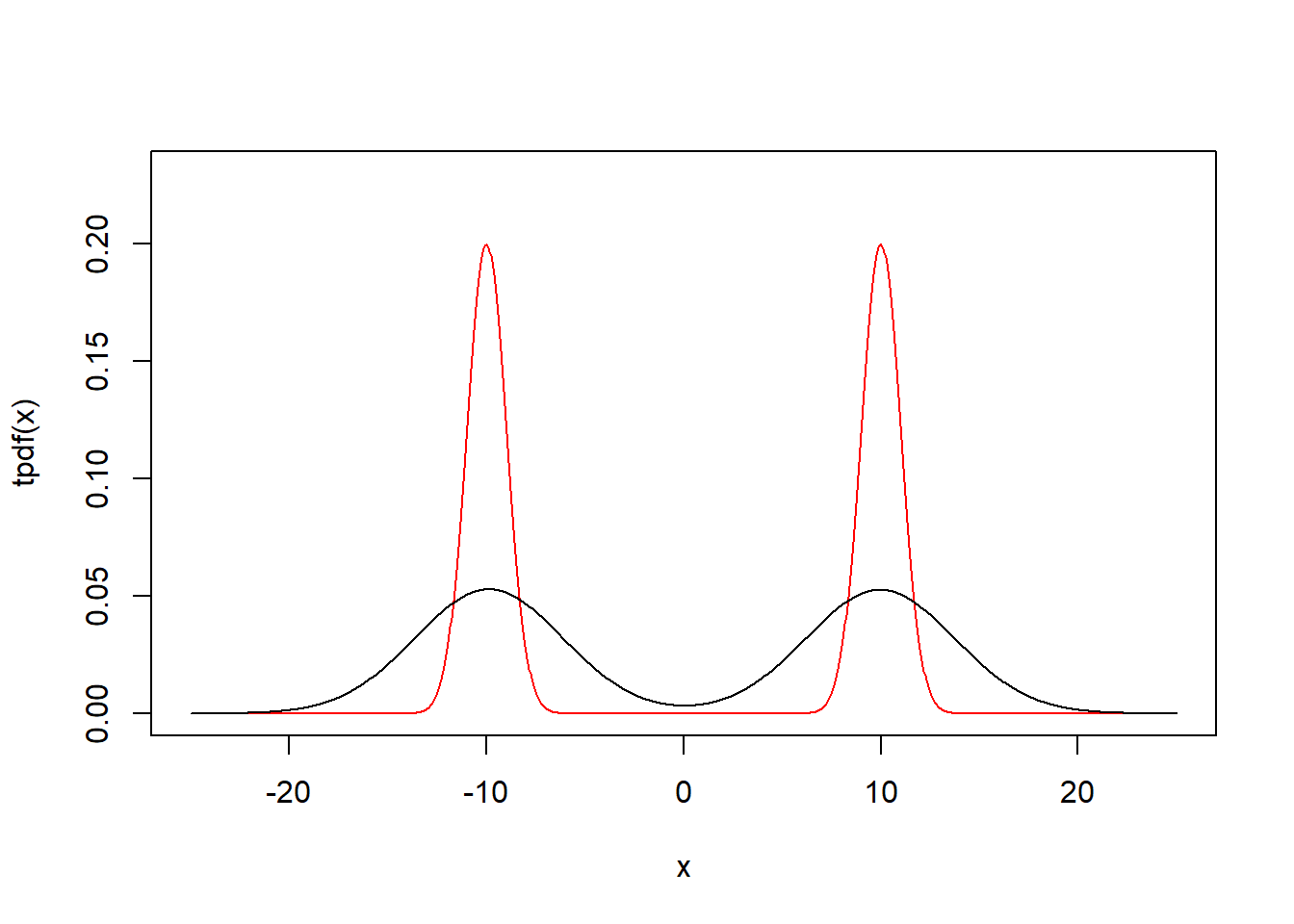
plot(x,tpdf(x),type="l",ylim=c(0,0.23),col="red")
par(new=T)
plot(x,kpdf(x),type="l",ylim=c(0,0.23),xlab="",ylab="",axes=F)